All three terms are used to describe phenomena where large events are rare, but small ones quite common. For example, there are few large earthquakes but many small ones. There are a few mega-cities, but many small towns. There are few words, such as 'and' and 'the' that occur very frequently, but many which occur rarely.

Zipf's law usually refers to the 'size' y of an occurrence of an event relative to it's rank r. George Kingsley Zipf, a Harvard linguistics professor, sought to determine the 'size' (or frequency of use in english text) of the 3rd or 8th or 100th most common word. Zipf's law states that the size of the r'th largest occurrence of the event is inversely proportional to it's rank:
y ~ r^-b, with b close to unity.

Pareto was interested in the distribution of income. Instead of asking what the r th largest income is, he asked how many people have an income greater than x. Pareto's law is given in terms of the cumulative distribution function (CDF), i.e. the number of events larger than x is an inverse power of x:
P[X > x] ~ x^-k.
It states that there are a few multi-billionaires, but most people make only a modest income.

What is usually called a power law distribution tells us not how many people had an income greater than x, but the number of people whose income is exactly x. It is simply the probability distribution function (PDF) associated with the CDF given by Pareto's Law. This means that
P[X = x] ~ x^-(k+1) = x^-a.
That is the exponent of the power law distribution a = 1+k (where k is the Pareto distribution shape parameter).
See Appendix 1 for discussion of Pareto and power-law.

Although the literature surrounding both the Zipf and Pareto distributions is vast, there are very few direct connections made between Zipf and Pareto, and when they exist, it is by way of a vague reference [1] or an overly complicated mathematical analysis[2,3]. Here I show a simple and direct relationship between the two by walking through an example using real data.

Recently, attention has turned to the internet which seems to display quite a number of power-law distributions: the number of visits to a site [4], the number of pages within a site [5], and the number of links to a page [6], to name a few. My example will be the distribution of visits to web sites.

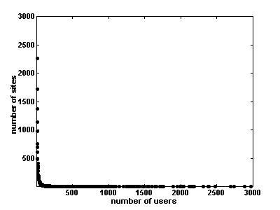
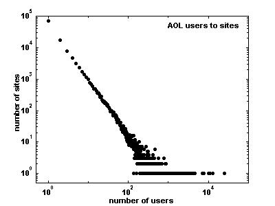
Figure 1a below shows the distribution of AOL users' visits to various sites on a December day in 1997. One can observe that a few sites get upward of 2000 visitors, whereas most sites got only a few visits (70,000 sites received only a single visit). The distribution is so extreme that if the full range was shown on the axes, the curve would be a perfect L shape. Figure 1b below shows the same plot, but on a log-log scale the same distribution shows itself to be linear. This is the characteristic signature of a power-law.

Fig. 1a Linear scale plot of the distribution of users among web sites	Fig. 1b Log-log scale plot of the distribution of users among web sites

Let y = number of sites that were visited by x users.
In a power-law we have y = C x^-a which means that log(y) = log(C) - a log(x)
So a power-law with exponent a is seen as a straight line with slope -a on a log-log plot.

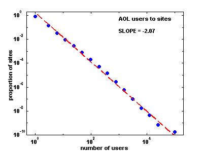
Now one just might be tempted to fit the curve in Fig. 1b to a line to extract the exponent a. A word of caution is in order here. The tail end of the distribution in Fig. 1b is 'messy' - there are only a few sites with a large number of visitors. For example, the most popular site, Yahoo.com, had 129,641 visitors, but the next most popular site had only 25,528. Because there are so few data points in that range, simply fitting a straight line to the data in Fig. 1b gives a slope that is too shallow (a = 1.17). To get a proper fit, we need to bin the data into exponentially wider bins (they will appear evenly spaced on a log scale) as shown in Fig. 2. A clean linear relationship now extends over 4 decades (1-10⁴) users vs. the earlier 2 decades: (1-100) users. We are now able to extract the correct exponent a = 2.07.

Fig. 2 Binned distribution of users to sites

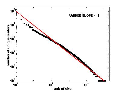
So far we have only looked at the power-law PDF of sites visits. In order to see Zipf's law, we need to plot the number of visitors to each site against its rank. Fig. 3 shows such a plot for the same data set of AOL users' site visits. The relationship is nearly linear on a log-log plot, and the slope is -1, which makes it Zipf. In order for there to be perfectly linear relationship, the most popular sites would have to be slightly popular, and the less popular sites slightly more numerous. It might be worthwhile to fit this distribution with alternate distributions, such as the stretched exponential [7], or parabolic fractal [8]. In any case, most would happy to call this rank distribution Zipf, and we will call it Zipf here as well.

Fig. 3 Sites rank ordered by their popularity

At first, it appears that we have discovered two separate power laws, one produced by ranking the variables, the other by looking at the frequency distribution. Some papers even make the mistake of saying so [9]. But the key is to formulate the rank distribution in the proper way to see its direct relationship to the Pareto. The phrase "The r th largest city has n inhabitants" is equivalent to saying "r cities have n or more inhabitants". This is exactly the definition of the Pareto distribution, except the x and y axes are flipped. Whereas for Zipf, r is on the x-axis and n is on the y-axis, for Pareto, r is on the y-axis and n is on the x-axis. Simply inverting the axes, we get that if the rank exponent is b, i.e.
n ~ r^-b in Zipf,   (n = income, r = rank of person with income n)
then the Pareto exponent is 1/b so that
r ~ n^-1/b   (n = income, r = number of people whose income is n or higher)
(See Appendix 2 for details).

Of course, since the power-law distribution is a direct derivative of Pareto's Law, its exponent is given by (1+1/b). This also implies that any process generating an exact Zipf rank distribution must have a strictly power-law probability density function. As demonstrated with the AOL data, in the case b = 1, the power-law exponent a = 2.

Finally, instead of touting two separate power-laws, we have confirmed that they are different ways of looking at the same thing.

Acknowledgements

References

1. Per Bak, "How Nature Works: The science of self-organized criticality", Springer-Verlag, New York, 1996.

2. G. Troll and P. beim Graben (1998), "Zipf's law is not a consequence of the central limit theorem", Phys. Rev. E, 57(2):1347-1355.

3. R. Gunther, L. Levitin, B. Shapiro, P. Wagner (1996), "Zipf's law and the effect of ranking on probability distributions", International Journal of Theoretical Physics, 35(2):395-417

4. L.A. Adamic and B.A. Huberman (2000), "The Nature of Markets in the World Wide Web", QJEC 1(1):5-12.

5. B.A. Huberman and L.A. Adamic (1999), "Growth Dynamics of the World Wide Web", Nature 401:131.

6. R. Albert, H. Jeoung, A-L Barabasi, "The Diameter of the World Wide Web", Nature 401:130.

7. Jean Laherrere, D Sornette (1998), "Stretched exponential distributions in Nature and Economy: 'Fat tails' with characteristic scales", European Physical Journals, B2:525-539. http://xxx.lanl.gov/abs/cond-mat/9801293

8. Jean Laherrere (1996), "'Parabolic fractal' distributions in Nature".

9. M. Faloutsos, P. Faloutsos, and C. Faloutsos, "On Power-Law Relationships of the Internet Topology", SIGCOMM '99 pp. 251-262.

10. N. Johnson, S. Kotz, N. Balakrishnan, "Continuous Univariate Distributions Vol. 1", Wiley, New York, 1994.

Appendix 1: The Pareto Distribution

Another property, which holds for all k, not just those k not giving a finite mean, is that the distribution is said to be "scale-free", or lacking a "characteristic length scale". This means that no matter what range of x one looks at, the proportion of small to large events is the same, i.e., the slope of the curve on any section of the log-log plot is the same.

Appendix 2: From Zipf's ranked distribution to powerlaw PDFs

Let the slope of the ranked plot be b.

Then the expected value E[X_r ] of the rth ranked variable X_r is given by

E[X_r ] ~ C₁*r^-b,     C₁ a normalization constant,

which means that there are r variables with expected value greater than or equal to C₁*r^-b:

P[X >= C₁*r^-b] = C₂*r

Changing variables we get:

P[X >= y] ~ y^-(1/b)

To get the PDF from the CDF, we take the derivative with respect to y:

Pr[X == y] ~ y^-(1+(1/b)) = y^-a.

Which gives the desired correspondence between the two exponents.

a = 1+(1/b)